10 Simulation
Random numbers can be used for:
- simulation of complex systems
- encryption
- bootstrap methods (the bootstrap method is a resampling technique used to estimate statistics on a population by sampling a dataset with replacement. It can be used to estimate summary statistics such as the mean or standard deviation \(\Longrightarrow\) Risk models course)
- design of experiments
- performance testing
- simulation testing of models and estimation
- …
How do we get random numbers?
- Use a natural phenomena. E.g: a dice, a deck of cards, …
- Use a table of random numbers.
- Computer algorithm: easy, but the algorithm should be:
- carefully selected
- fast
- simple
- reproducible
Item 3 is included in R. It is easy to simulate from most distributions of interest!
- Random numbers (in R) are actually called pseudo-random numbers (because the algorithm can repeat the sequence, and the numbers are thus not entirely random).
- Generated from an algorithm.
- For all practical purposes, pseudo-random numbers behave like true random numbers.
- By specifying the input to the algorithm, pseudo-random numbers can be re-created.
- The default pseudo random number generator in R is the Mersenne Twister.
- In R the Mersenne Twister uses a random seed as input: constructed from time and session ID.
- You can replace the random seed with a fixed seed with the
set.seed()function.
10.1 The set.seed()function
- Sets of random numbers:
> set.seed(12345)
> rnorm(3)
## [1]  0.5855  0.7095 -0.1093
> rnorm(5)
## [1] -0.4535  0.6059 -1.8180  0.6301 -0.2762
> rnorm(3)
## [1] -0.2842 -0.9193 -0.1162
As an exercise follow the steps:
1 - Save your work, close RStudio and open it again.
2 - Run:
3 - Save the 5 numbers.
4 - Close RStudio and open it again.
5 - Run:
6 - Repeat the exercise with a different seed at point 5.
10.2 Random numbers and probability distributions
Very useful link.
- Simulation from a uniform distribution:
- Simulation from a normal distribution:
- Simulation from a gamma distribution:
- Simulation from a binomial distribution:
- Simulation from a multinomial distribution:
> rmultinom(5,size=100,prob=c(.3,.2,.5))
##      [,1] [,2] [,3] [,4] [,5]
## [1,]   24   27   30   30   37
## [2,]   15   21   16   20   13
## [3,] 61 52 54 50 50- List of functions:
> # Density -> d
> dnorm(x, mean = 0, sd = 1, log = FALSE)
>
> # Distribution function -> p
> pnorm(q, mean = 0, sd = 1, lower.tail = TRUE, log.p = FALSE)
>
> # Quantile function -> q
> qnorm(p, mean = 0, sd = 1, lower.tail = TRUE, log.p = FALSE)
>
> # Random generator -> r
> rnorm(n, mean = 0, sd = 1)- Remember…
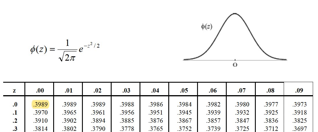
Figure 10.1: Standard Gaussian distribution.
- Distributions:
>
> # normal: dnorm(x=..., mean=..., sd=...); x is a quantile.
>
> # dnorm(0,0,1) = 1/sqrt(2*pi)
> dnorm(0,0,1)
## [1] 0.3989
> dnorm(0,0,1) == 1/sqrt(2*pi)
## [1] TRUE
>
> # normal: pnorm(q=..., mean=..., sd=...); q is a quantile.
> pnorm(0,0,1)
## [1] 0.5
> pnorm(-1.96,0,1)
## [1] 0.025
> pnorm(-1.64,0,1)
## [1] 0.0505
> pnorm(1.96,0,1)
## [1] 0.975
> pnorm(1.64,0,1)
## [1] 0.9495
>
> # normal: qnorm(p=..., mean=..., sd=...); p is a probability.
> qnorm(0.5,0,1)
## [1] 0
> qnorm(0.95,0,1)
## [1] 1.645
> qnorm(0.975,0,1)
## [1] 1.96
10.3 Monte Carlo integration (example)
- Consider the function \(f(x)=e^{2\cos(x-\pi)}\) and compute the integral \[\int\limits_0^{2\pi} f(x) dx:\]
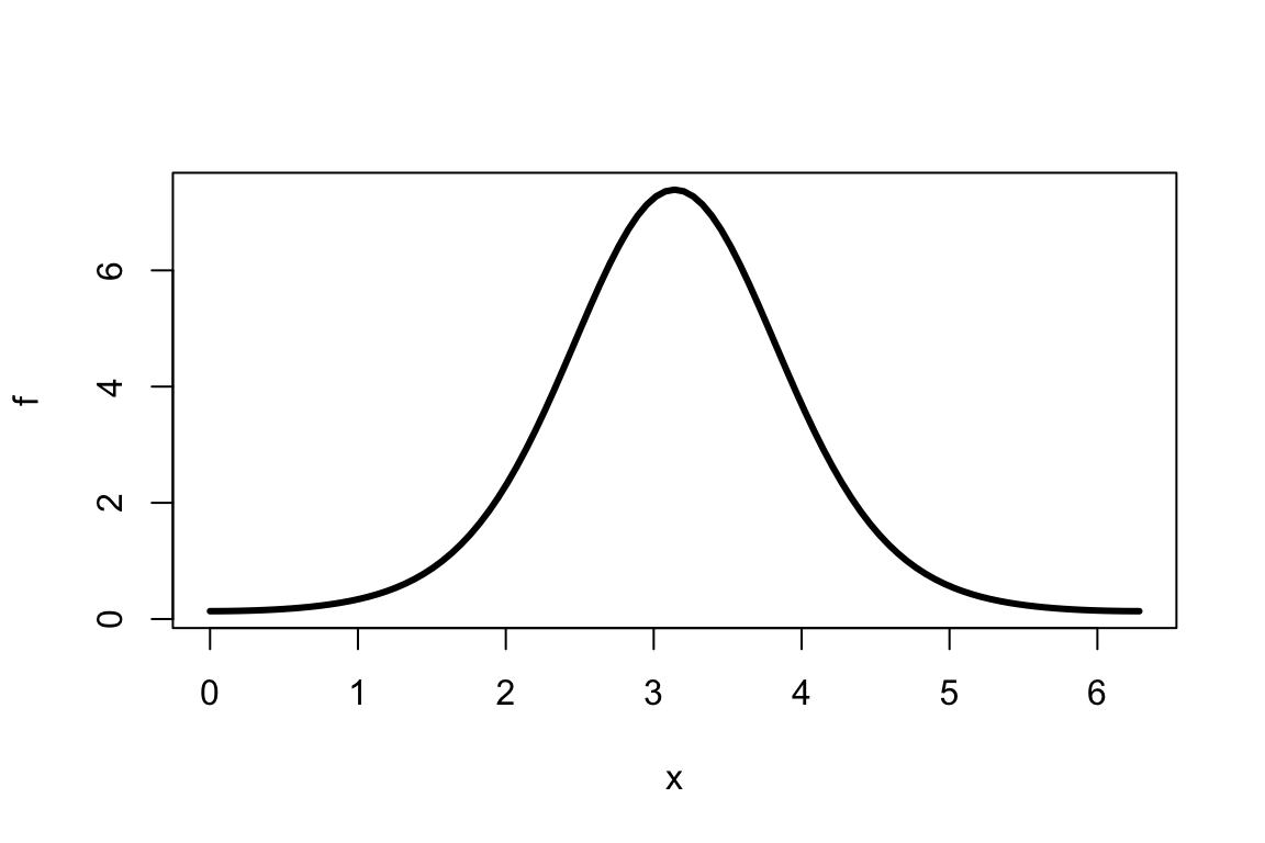
- Monte Carlo method:
- simulate uniformly distributed points \((x_1,~y_1), \ldots, (x_n,~y_n)\) in \([0, ~2\pi] \times [0,~8]\) within a “box”. Note that \(0<f(x)<e^{2}, ~\forall ~x \in [0, ~2\pi]\):
> set.seed(1234)
> plot(f, 0, 2*pi, lwd=3)
> x<-runif(1000,0,2*pi)
> y<-runif(1000,0,exp(2))
> mycol<-ifelse(y<f(x),'blue','green')
> points(x,y,col=mycol)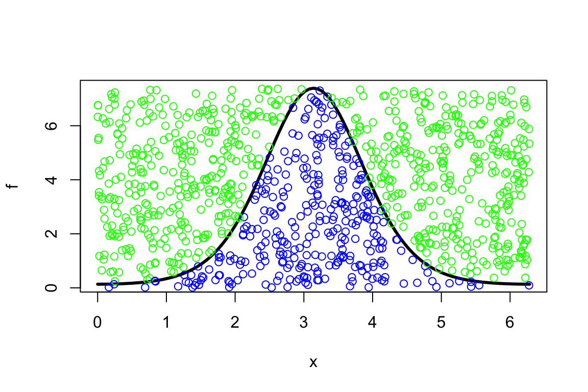
(to get a wider view of what’s happening:)
> set.seed(1234)
> plot(f, 0, 2*pi, xlim=c(-1,10), ylim=c(-1,10), lwd=3)
> x<-runif(1000,0,2*pi)
> y<-runif(1000,0,exp(2))
> mycol<-ifelse(y<f(x),'blue','green')
> points(x,y,col=mycol)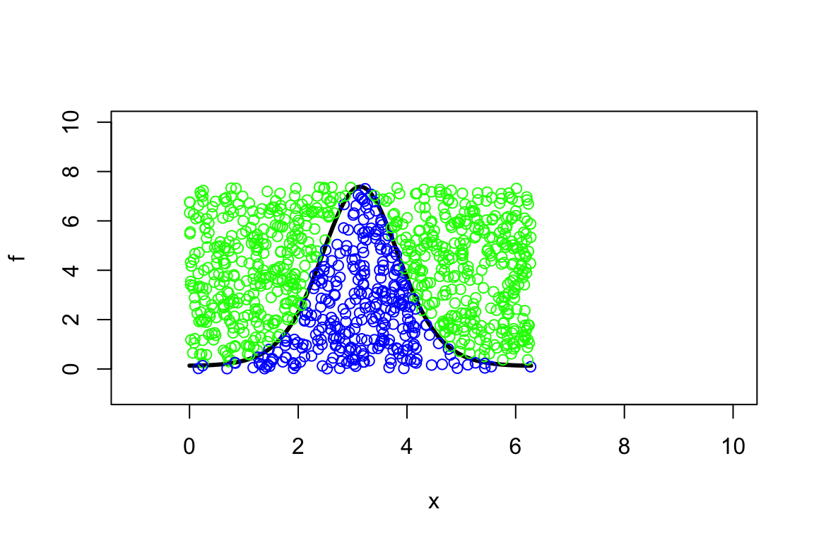
- estimate the probability of points (say \(m\)) being below the curve of \(f\): \(m/n\).
- the area of the “box” is \(2\pi \times e^2 \approx 46.43\), so the estimated integral, i.e., the area under the curve, becomes \[\int\limits_0^{2\pi} f(x) dx \approx 46.43 \times \frac{m}{n}.\]
> set.seed(4321)
>
> x<-runif(1e+06,0,2*pi)
> y<-runif(1e+06,0,exp(2))
> m.over.n<-sum(y<f(x))/length(x)
>
> options(digits=20)
> (MCint <- m.over.n*46.43)
## [1] 14.325558629999999738
>
> # "real" value
> (Realint <- integrate(f,0,2*pi)$value)
## [1] 14.323056878100514311
>
> (MCint-Realint)
## [1] 0.0025017518994854270886
>
> options(digits=4)