11 Linear models

• Statistical models of a linear relationship between variables: \[Y=\beta_0+\beta_1X+e,\] where:

  • \(Y\) is the dependent variable;
  • \(X\) is the independent variable;
  • \(e\) is the error term;

• The errors should be independent, identically normally distributed, with mean \(0\) and variance \(\sigma^2>0\).

• The model parameters to be estimated are: \(\beta_0\) and \(\beta_1\).

• Examples: \(\hat y=1+0.5x\), \(\hat y=0-2x\).

• In R: consider 1000 pairs \((x_i,y_i)\) as follows

> set.seed(98765421)
> x<-rchisq(1000,df=1)
> y<-1+0.5*x+0.7*rnorm(1000)
> 
> plot(x,y,xlab='x',ylab='y')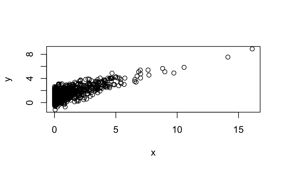

• The main idea is to compute the best linear model, that is, the best blue line:

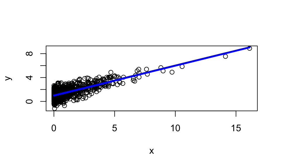
• Suppose the estimated model \(\hat y=1+0.5x\) for the above data.

• Model residuals:

> residuals.y<-y-(1+0.5*x)
> 
> # Check assumptions
> f<-function(x){dnorm(x,sd=sd(residuals.y))}
> hist(residuals.y,probability=TRUE,ylim=c(0,0.7),nclass = 20)
> curve(f,col="blue", lwd=3, add=TRUE)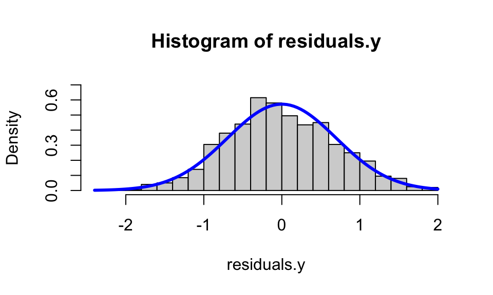

11.1 Fitting models: the lm()function

\[y=\beta_0+\beta_1x+e\]

• In R linear models can be fitted to data with the lm() function:

> analysis<-lm(y~x)
> analysis
## 
## Call:
## lm(formula = y ~ x)
## 
## Coefficients:
## (Intercept)            x  
##       0.991        0.496

• So, parameter estimates are: \(\hat{\beta}_0=0.991\) and \(\hat{\beta}_1=0.496\).

• Model formulas: the argument to lm() is a formula object. A linear model is specified by a formula object, which may look like this:

> my.formula<-formula(y~x+z+w)
> fit<-lm(my.formula)
> # or
> fit<-lm(y~x+z+w)

• The corresponding linear model is: \[y=\beta_0+\beta_1x+\beta_2z+\beta_3w+e.\]

• Contents of the lm() function:

> analysis<-lm(y~x)
> names(analysis)
##  [1] "coefficients"  "residuals"     "effects"       "rank"         
##  [5] "fitted.values" "assign"        "qr"            "df.residual"  
##  [9] "xlevels"       "call"          "terms"         "model"

• Accessing the contents:

> analysis$coef
## (Intercept)           x 
##      0.9909      0.4964

• Summaries:

> summary(analysis)
## 
## Call:
## lm(formula = y ~ x)
## 
## Residuals:
##     Min      1Q  Median      3Q     Max 
## -2.2027 -0.4663 -0.0532  0.5073  1.9379 
## 
## Coefficients:
##             Estimate Std. Error t value Pr(>|t|)    
## (Intercept)   0.9909     0.0267    37.1   <2e-16 ***
## x             0.4964     0.0142    35.0   <2e-16 ***
## ---
## Signif. codes:  0 '***' 0.001 '**' 0.01 '*' 0.05 '.' 0.1 ' ' 1
## 
## Residual standard error: 0.698 on 998 degrees of freedom
## Multiple R-squared:  0.551,  Adjusted R-squared:  0.551 
## F-statistic: 1.23e+03 on 1 and 998 DF,  p-value: <2e-16

---